The study of cellular dynamics through mathematical modeling is a crucial area of research for understanding tumor progression. Diffusion equations, in particular, provide a powerful framework for modeling the global behavior arising from complex microscopic processes. These models not only describe the evolution of cell populations structured by age and size but also facilitate the formulation of relevant mathematical control strategies in the context of tumor biology. In this study, we focus on exploring null controllability within the framework of population dynamics, incorporating age and size structuring along with diffusion effects. The goal is to make a theoretical contribution by demonstrating how these models can offer new insights into the regulation of cellular dynamics. While the potential application to cancer therapy is an underlying motivation, our approach is centered on the mathematical foundations necessary for understanding and analyzing the underlying biological phenomena.

We consider the following system \[\left\lbrace\begin{array}{ll} \dfrac{\partial y}{\partial t}+\dfrac{\partial y}{\partial a}+\dfrac{\partial (g(s)y) }{\partial s}-\Delta y+\mu(a,s)y=0 &\hbox{ in }\Omega\times (0,A)\times (0,S)\times(0,+\infty) ,\\ \dfrac{\partial y}{\partial \nu}=0&\hbox{ }(x,a,s,t)\in\partial\Omega\times(0,A)\times (0,S)\times(0,\infty),\\ y\left(x,0,s,t\right) =y_{i}(x,s,t)&\hbox{ } (x,s,t)\in\Omega\times (0,S)\times(0,\infty) \\ y\left(x,a,s,0\right)=y_{0}\left(x,a,s\right)& \hbox{ }(x,a,s)\in \Omega\times(0,A)\times (0,S);\\ y(x,a,0,t)=0& \hbox{ } (x,a,t)\in\Omega\times(0,A)\times(0,\infty). \end{array}\right. \label{2}\] where \(y(x,a,s,t)\) (carcinogenic cells) is a distribution of individuals of age \(a\) size \(s\) at time \(t\) and location \(x\in\Omega\). \(A\) and \(S\) are respectively the maximal live expectancy and the maximal size, \(\mu(a,s)\) natural death rate of individuals of individual.
\(\dfrac{\partial y}{\partial a}\) is the aging
\(\dfrac{\partial (g(s)y) }{\partial s}\) is the growing
\(\mu(a,s)y\) is the damping
\(y_i(x,s,t) \hbox{, }i\in\{1,2\}\) is the birth the rate, here we consider two type of birth rate.
\[y^{1}_{1}(x,s,t)=\displaystyle\int\limits_{0}^{A}\int\limits_{0}^{S}\beta_1(a,\hat{s},s)y(x,a,\hat{s},t)da d\hat{s}.\] Here \(\beta_1\) is a positive function describing the fertility rate age-size, which depends on \((a,\hat{s})\) and also depending on the size \(s\) of the newborns.
In probabilistic terms, fertility \(\beta_1\) can mean the probability of an individual of age \(a\) and of size \(\hat{s}\) giving birth to an individual of size \(s.\) and
\[y^{1}_{2}(x,s,t)=\displaystyle\int\limits_{0}^{A}\beta_2(a,s)y(x,a,s,t)da\]
It is assumed that size increases in the same way for everyone in the population and is controlled by the growth function \(g(s),\) then \(\dfrac{\partial (g(s)y) }{\partial s}\) is the growth.
Description of age and size structured model According to Gleen Webb, if the mortality and fertility rates \(\mu(a,s)=\mu_1(a)+\mu_2(s)\) and \(\beta_i\) are such that:
[overleaf] \[\begin{aligned} ( {\bf H1}):& \left\lbrace \begin{array}{l} \mu_1(a)\geq 0 \text{ for every } a\in (0,A)\\ \mu_1\in L^{1}\left([0,a^*]\right)\hbox{ for every }\; a^*\in [0,A) \\ \displaystyle\int\limits_{0}^{A}\mu_1(a)da=+\infty \end{array} \right. ,\quad ( {\bf H2}): \left\lbrace\begin{array}{l} \mu_2(s)\geq 0 \hbox{ for every } s\in (0,S)\\ \mu_2\in L^{1}\left([0,s^*]\right)\hbox{ for every }\hbox{ } s^*\in [0,A) \\ \displaystyle\int\limits_{0}^{S}\mu_2(s)ds=+\infty \end{array} \right.\cr ( {\bf H3}):& \left\lbrace\begin{array}{l} g(x)>0\hbox{ for all }x\in [0,S]\hbox{ and }g\in C^1([0,S]);\\ %\int\limits_{a}^{b}\dfrac{ds}{g(s)}<+\infty \hbox{ for all }[a,b]\subset [0,S]. \end{array} \right. \qquad ( {\bf H4}): \left\lbrace\begin{array}{l} \beta_i \hbox{ is continuous }i\in \{1,2\}\\ \beta_i\geq0 \hbox{, } i\in \{1,2\}\\ \end{array} \right. \qquad\end{aligned}\] \[\begin{aligned} ({\bf H5}): \begin{array}{c} \beta_i(a,.)=0 \text{ } \forall a\in (0,\hat{a}) \text{ for some } \hat{a}\in (0,A)\hbox{ and }i\in \{1,2\}. \end{array}\end{aligned}\]
for any initial condition \(y_0\in K=L^2\left(\Omega\times (0,A)\times (0,S)\right),\) the system \((1)\) admits a unique solution.
We consider the following system \[\left\lbrace\begin{array}{ll} \dfrac{\partial y}{\partial t}+\dfrac{\partial y}{\partial a}+\dfrac{\partial (g(s)y) }{\partial s}-\Delta y+\mu(a,s)y=u\chi_{\Theta} &\hbox{ in }\Omega\times (0,A)\times (0,S)\times(0,\infty) ,\\ \dfrac{\partial y}{\partial \nu}=0&\hbox{ }(x,a,s,t)\in\partial\Omega\times(0,A)\times (0,S)\times(0,\infty),\\ y\left(x,0,s,t\right) =y^{1}_{i}(x,s,t)&\hbox{ } (x,s,t)\in\Omega\times (0,S)\times(0,\infty)\hbox{, }i\in\{1,2\} \\ y\left(x,a,s,0\right)=y_{0}\left(x,a,s\right)& \hbox{ }(x,a,s)\in \Omega\times(0,A)\times (0,S);\\ y(x,a,0,t)=0& \hbox{ } (x,a,t)\in\Omega\times(0,A)\times(0,\infty). \end{array}\right. \label{2a}\] where
\(\Theta=\omega\times(a_1,a_2)\times (s_1,s_2)\);
\(u(x,a,s,t)\) is the control;
\(\omega\times(a_1,a_2)\times (s_1,s_2)\subset \Omega\times (0,A)\times (0,S)\) is the support of the control;
Goal: To drive the solution to equilibrium at a given final time \(T>0\) \[y(.,.,.,T)\equiv 0\]
Since the controllability of the linear system is equivalent to an observability inequality, we consider the adjoint system: \[\left\lbrace\begin{array}{ll} \dfrac{\partial q}{\partial t}-\dfrac{\partial q}{\partial a}-g(s)\dfrac{\partial q}{\partial s}-\Delta q+\mu(a,s)q=q_i(x,s,t)&\hbox{ in }\Omega\times(0,A)\times (0,S)\times(0,+\infty) i\in\{1,2\},\\ \dfrac{\partial q}{\partial \nu}=0&\hbox{ }(x,a,s,t)\in\partial\Omega\times(0,A)\times (0,S)\times(0,\infty),\\ q\left( x,A,s,t\right) =0&\hbox{ in } (x,s,t)\in\Omega\times (0,S)\times(0,\infty) \\ q(x,a,S,t)=0& \hbox{ in } (x,a,t)\in\Omega\times(0,A)\times (0,\infty)\\ q\left(x,a,s,0\right)=q_0(x,a,s)& \hbox{ in }(x,a,s)\in\partial\Omega\times(0,A)\times (0,S); \end{array}\right.\] with the following correspondence \[q_1(x,s,t)=\displaystyle\int\limits_{0}^{S}\beta_1(a,s,\hat{s})q(x,0,\hat{s},t)d\hat{s}\hbox{ matches with }y^{1}_{1},\] and \[q_2(x,s,t)=\beta_2(a,s)q(x,0,s,t)\hbox{ matches with }y^{1}_{2}.\]
The null controllability problem therefore becomes an observability inequality problem and the question is whether: is the inequality \[\displaystyle\int\limits_{0}^{S}\int\limits_{0}^{A}\int_{\Omega}q^2(a,s,T)dxdads\leq K_T\displaystyle\int\limits_{0}^{T}\int\limits_{s_1}^{s_2}\int\limits_{a_1}^{a_2}\int_{\omega}q^2(a,s,t)dadsdt.\] verified? The observation being made in the subset \[\omega\times(a_1,a_2)\times (s_1,s_2)\subset \Omega\times (0,A)\times (0,S).\]
The answer to the previous question is affirmative and we have the following null controllability result.
We denote by \[S^{*}_{1}=\int\limits_{0}^{s_1}\dfrac{ds}{g(s)}\hbox{, }S^{*}_{2}=\int\limits_{s_2}^{S}\dfrac{ds}{g(s)}\hbox{ and }T_0=\max\{S^{*}_{1},S^{*}_{2}\}\] and \[T_1=\max\left\{a_1+S^{*}_{2},S^{*}_{1}\right\}.\]
The null controllability result holds in \[\omega\times(a_1,a_2)\times (s_1,s_2)\subset \Omega\times (0,A)\times (0,S)\] with \(a_1<\hat{a}\), \[S^{*}_{2}<\min\{a_2-a_1,\hat{a}-a_1\}\hbox{ and }S^{*}_{1}<\min\{a_2,\hat{a}\}\] provided the fertility rate is such that \[\beta_i(a,.)\equiv 0\hbox{ in }(0,a_1+\gamma),\] and the time T is large enough such that:
for the birth rate equal \(y^{1}_{1}\), \(T>A-a_2+T_1+T_0\) and
for the birth rate equal \(y^{1}_{2}\), \(T>A-a_2+a_1+S_1^*+S_2^*.\)
The proof of the observability inequality is based on the estimation of the non-local term \(q_i\hbox{, }i\in\{1,2\}\).
As \[\beta_i(a,.)\equiv 0\hbox{ in }(0,a_1+\gamma),\] the first equation of the adjoint system become \[\dfrac{\partial q}{\partial t}-\dfrac{\partial q}{\partial a}-g(s)\dfrac{\partial q}{\partial s}-\Delta q+\mu(a,s)q=0\hbox{ in }\Omega\times(0,\hat{a})\times (0,S)\times(0,+\infty).\] We denote by \[\tilde{q}(x,a,s,t)=q(x,a,s,t)\exp\left(-\int\limits_{0}^{a}\mu_1(\alpha)d\alpha-\int\limits_{0}^{s}\mu_2(r)dr\right).\]\[w(x,\lambda)=\tilde{q}(x,t,G^{-1}(G(s)+t),0) \text{ ; }x\in\Omega\hbox{, }\lambda\in (0,t).\]
Then \(w\) satisfies:
\[\dfrac{\partial w(x,\lambda)}{\partial \lambda}-\Delta w(x,\lambda)=0\text{ in } \Omega\times (0,t).\]
Then the sum \(q_{1}\) can be estimate for all time \(t>T_1.\)
And the term \(q_{2}\) can be estimate for all time \(t>T_1.\)
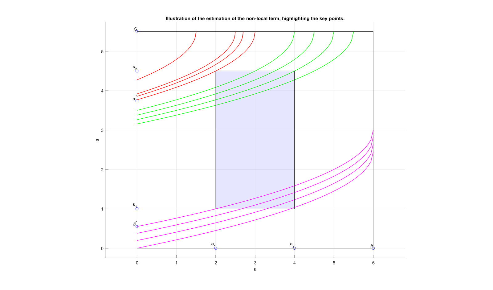

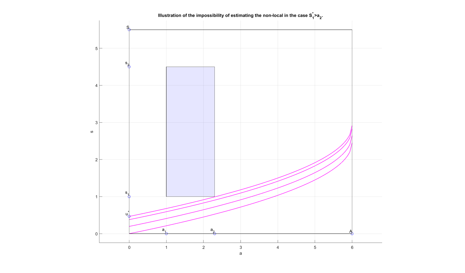

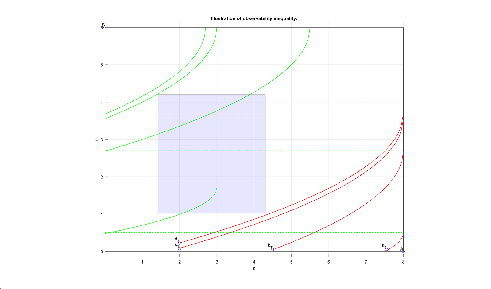
Interpretation of Constraints (see Figure 2-3 below) Condition \(S^*_1 < \min\{a_2,\hat{a}\}<\hat{a}\) means that all newborns must reach size \(s_1\) before age \(\hat{a}\) (reproductive age). This imposes an appropriate choice of the bound \(s_1\). Condition \(S^*_2 + a_1 < \hat{a}\) means that all newborns who exceed size \(s_2\) before age \(a_1\) must reach maximum size \(S\) before the age of fertility \(\hat{a}\). This imposes an appropriate choice of the bound \(s_2\). An explanation of the control time for this problem is as follows. Interpretation of the result within the context of a positivity constraint from a heuristic perspective (see Figure 1-2): In this interpretation, we acknowledge that at \(t = 0\), individuals of all ages and sizes may be present. We focus on controlling individuals whose age falls between \(a_1\) and \(a_2\) and whose size falls between \(s_1\) and \(s_2\). The extreme scenario assumes that any individual meeting the control criteria is automatically eliminated (extreme control with a positivity constraint). For individuals existing before the control period, they may grow without reaching the size and age thresholds for elimination. However, individuals born after the start of the control period will either be eliminated upon reaching the threshold or may not reach the age required for reproduction before perishing (\(S_{1}^* < \max\{a_2, \hat{a}\}\) and \(S_{2}^* < \max\{a_2, \hat{a}\}\)). Two situations may arise:
An individual (with size less than \(s_1\)) born just before the control period may survive for approximately \(G(s_1)\) time units plus \(A - a_2\) time units before dying. Before their demise, this individual may give birth to offspring of all sizes, who will have at most \(T_1\) time units before being eliminated or dying. The total lifespan of this individual and their offspring is therefore \(A - a_2 + S_{1}^* + T_1\).
An individual whose size exceeds \(s_2\) can live for around \(S_{2}^*\) time units plus \(A - a_2\) time units before dying. Before their death, this individual may give birth to offspring of all sizes, who will have at most \(T_1\) time units before being eliminated. The total lifespan of this individual and their offspring is \(A - a_2 + S_{2}^* + T_1\).
In conclusion, the overarching condition set by these scenarios is \(T > (A - a_2) + T_0 + T_1\). This condition encapsulates the collective times considered regarding the age constraint, the survival periods before and after control, and the limited lifespan of individuals born during or after the control period in the extreme feedback control mechanism outlined in the provided explanation. The two figures below highlight two key aspects of the result: . The impact of the random size of newborns on the estimated controllability time. Specifically, the size at birth dictates a trajectory that must be followed to reach the control threshold.. A heuristic method to estimate the controllability time. Moreover, the figures illustrate the controllability time in the case of extreme control with positivity constraint.

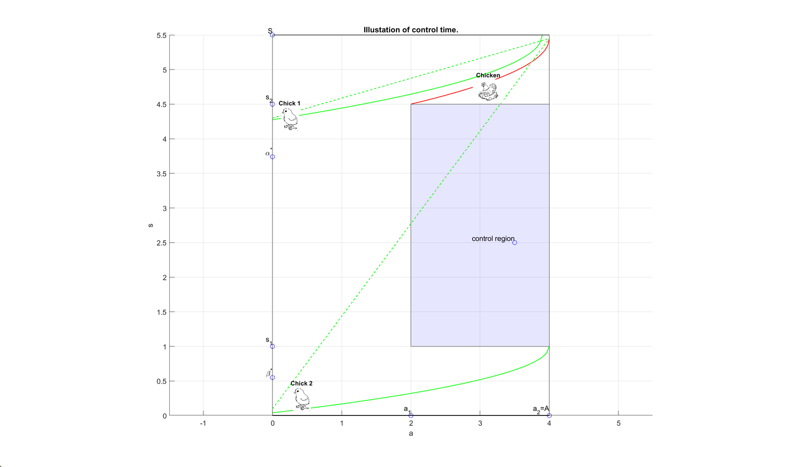
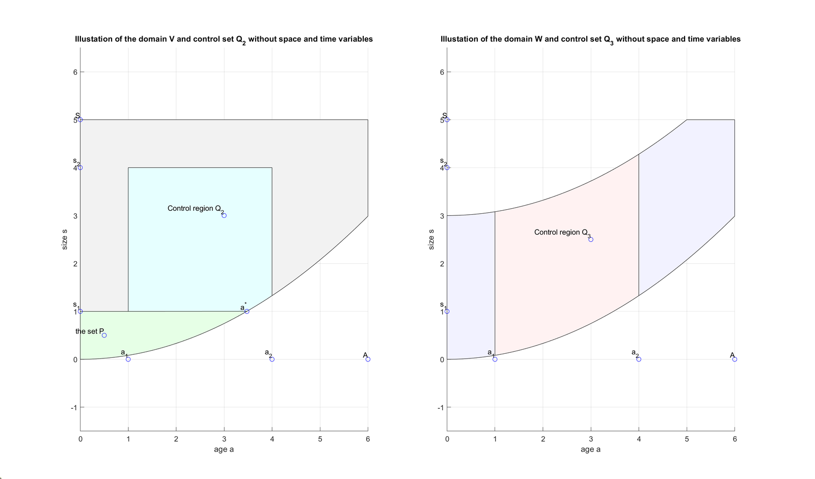
Analysis of the case where individuals aged \(a \in (0,A)\) have a size \(s\) satisfying \(G^{-1}(a) \leq s \leq S\) at the initial time (refer to Figure 3). By assuming that size increases uniformly for all individuals in the population and is determined by the growth function \(g(s)\), the study domain of the model can be confined to the following: \[V = \{(x,a,s,t) \in \Omega \times (0,A) \times (0,S) \times (0,T) \;|\; 0 \leq a \leq A;\; G^{-1}(a) \leq s \leq S;\; 0 \leq t \leq T \}.\] Therefore, no individual of age \(a\) and size \(s\) falls into the domain: \[W = \{(x,a,s,t) \in \Omega \times (0,A) \times (0,S) \times (0,T) \;|\; 0 \leq a \leq A;\; 0 \leq s < G^{-1}(a);\; 0 \leq t \leq T \}.\] Assuming \(V\) to be the study domain and considering the control set: \[Q_2 = \{(x,a,s,t) \in Q \;|\; x \in \omega, \; a_1 \leq a \leq a_2, \; \max\{s_1,G^{-1}(a)\} \leq s \leq s_2, \; 0 \leq t \leq T \},\] (refer to Figure 3), then the estimated time \(T\) must satisfy: \[T > A - a_2 + T_1 + S^*_2.\] In addition, this result is achieved without the condition \(S^*_1 < a_2\). A detailed proof for this scenario will be presented at the end of this part. Furthermore, if newborns’ size cannot exceed \(s_e\) such that each individual can reach fertility age without surpassing the maximum size \(S\), the domain \(V\) is redefined as: \[V = \{(x,a,s,t) \in \Omega \times (0,A) \times (0,S) \times (0,T) \;|\; 0 \leq a \leq A;\; G^{-1}(a) \leq s \leq G^{-1}(a+G(s_e));\; 0 \leq t \leq T \}.\] A control support can be outlined as: \[Q_3 = \{(x,a,s,t) \in Q \;|\; x \in \omega, \; a_1 \leq a \leq a_2, \; G^{-1}(a) \leq s \leq G^{-1}(a + G(s_e)), \; 0 \leq t \leq T\}.\] Consequently, in this scenario, the null controllability result is established without the constraints \(S^{*}_{2}<\min\{a_2-a_1,\hat{a}-a_1\}\) and \(S^{*}_{1}<\min\{a_2,\hat{a}\}\), with the condition \(T > a_1 + A - a_2\). These concepts are illustrated in the figure provided.
